Discussion
In my project, I determined through research and experimentation that a double pendulum is a chaotic system. In order to classify it as such, a double pendulum had to have three characteristics: dense periodic orbits, topologically mixing phase space, and high sensitivity to initial conditions.
Through research, I learnt that double pendulums have a dense periodic orbit. An orbit is collection of points that appear to show a pattern, and when the system is in a state in one orbit, it will never enter another orbit. A periodic orbit is an orbit that repeats. In a dense periodic orbit, every point in a chaotic system is arbitrarily close to a point on a periodic orbit – in other words, the periodic orbits are very dense around the points of the chaotic system and for any distance chosen from a chaotic point, there is a point on a periodic orbit within that distance. For a double pendulum, this means that no two pendulums will be the same, unless all its initial starting conditions were exactly identical and there was no perturbation whatsoever, which is highly improbable. Even though the pendulum may seem to be in a periodic orbit, repeating a pattern, or following the same pattern as another pendulum with different starting conditions (since it is so dense that we cannot tell), it is most likely not and its path could drastically alter any second.
Also through research, I learnt the double pendulums are topologically transitive. A phase space that is topologically mixing evolves over time so that any region of its phase space will eventually overlap with any other region. This means that any given point, no matter how far apart it is from another given point, will eventually end up arbitrarily close to it. For a double pendulum, this has a similar effect as a dense periodic orbit. Trajectories that are far apart could suddenly fall into a similar pattern.
For the actual experiment, I tested the sensitivity to initial conditions that a double pendulum has. The first part of my hypothesis stated if a system sensitive to initial starting conditions was dynamic, deterministic, and had a path greatly dependent on the starting conditions, then a double pendulum, a deterministic and dynamical system, with the abundance of possible states and its difficulty to recreate due to the second rod and mass, should be sensitive to initial starting conditions. To prove this, I tested the sensitivity of a double pendulum in three ways:
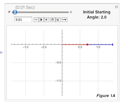
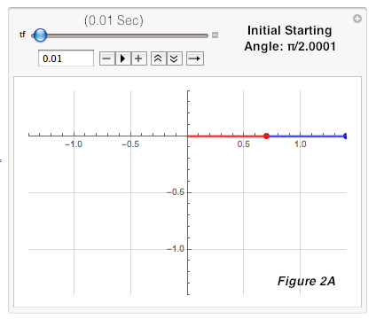
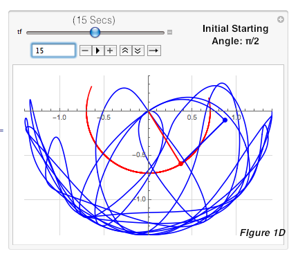
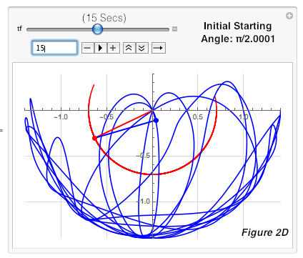
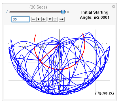
1) First, I used a parametric plot that simulated the path of the double pendulum, and recorded the 30-second paths for pendulums with initial starting angles of π/2 (as the control), π/2.0001, π/2.001, and π/2.01 in mass 1 and mass 2. I repeated each simulation three times to verify, and they remained consistent each time since the double pendulum is deterministic, and therefore only one trajectory can result from identical initial starting conditions. By observing the paths, I saw that most of the trajectories remained similar until about 10 seconds, after which they started visibly diverging. I took screenshots of these paths at 0.01, 5, 10, 15, 20, 25, and 30 for every pendulum, yielding Figures 1-4. As time passed, the pendulums became more and more different from π/2. For example, if you compared Figures 1A-1G to 2A-2G (which have an initial difference of only 0.0001), the trajectories start out similar but at 1D and 2D, visible diverges start forming and increase until 1G and 2G, where the differences are much more obvious. This proved that a double pendulum is sensitive to initial starting conditions, since the divergence between the trajectories grew from invisible to fairly obvious, and will continue to grow as time goes on. An increase in difference shows high sensitivity to initial starting conditions because unlike other systems in which a change is permanent but will remain constant, a small difference here in initial conditions will continue to grow and eventually have a large impact on the path of the pendulum.
Through research, I learnt that double pendulums have a dense periodic orbit. An orbit is collection of points that appear to show a pattern, and when the system is in a state in one orbit, it will never enter another orbit. A periodic orbit is an orbit that repeats. In a dense periodic orbit, every point in a chaotic system is arbitrarily close to a point on a periodic orbit – in other words, the periodic orbits are very dense around the points of the chaotic system and for any distance chosen from a chaotic point, there is a point on a periodic orbit within that distance. For a double pendulum, this means that no two pendulums will be the same, unless all its initial starting conditions were exactly identical and there was no perturbation whatsoever, which is highly improbable. Even though the pendulum may seem to be in a periodic orbit, repeating a pattern, or following the same pattern as another pendulum with different starting conditions (since it is so dense that we cannot tell), it is most likely not and its path could drastically alter any second.
Also through research, I learnt the double pendulums are topologically transitive. A phase space that is topologically mixing evolves over time so that any region of its phase space will eventually overlap with any other region. This means that any given point, no matter how far apart it is from another given point, will eventually end up arbitrarily close to it. For a double pendulum, this has a similar effect as a dense periodic orbit. Trajectories that are far apart could suddenly fall into a similar pattern.
For the actual experiment, I tested the sensitivity to initial conditions that a double pendulum has. The first part of my hypothesis stated if a system sensitive to initial starting conditions was dynamic, deterministic, and had a path greatly dependent on the starting conditions, then a double pendulum, a deterministic and dynamical system, with the abundance of possible states and its difficulty to recreate due to the second rod and mass, should be sensitive to initial starting conditions. To prove this, I tested the sensitivity of a double pendulum in three ways:
1) First, I used a parametric plot that simulated the path of the double pendulum, and recorded the 30-second paths for pendulums with initial starting angles of π/2 (as the control), π/2.0001, π/2.001, and π/2.01 in mass 1 and mass 2. I repeated each simulation three times to verify, and they remained consistent each time since the double pendulum is deterministic, and therefore only one trajectory can result from identical initial starting conditions. By observing the paths, I saw that most of the trajectories remained similar until about 10 seconds, after which they started visibly diverging. I took screenshots of these paths at 0.01, 5, 10, 15, 20, 25, and 30 for every pendulum, yielding Figures 1-4. As time passed, the pendulums became more and more different from π/2. For example, if you compared Figures 1A-1G to 2A-2G (which have an initial difference of only 0.0001), the trajectories start out similar but at 1D and 2D, visible diverges start forming and increase until 1G and 2G, where the differences are much more obvious. This proved that a double pendulum is sensitive to initial starting conditions, since the divergence between the trajectories grew from invisible to fairly obvious, and will continue to grow as time goes on. An increase in difference shows high sensitivity to initial starting conditions because unlike other systems in which a change is permanent but will remain constant, a small difference here in initial conditions will continue to grow and eventually have a large impact on the path of the pendulum.
|
|
|
|

|
|
2) Next, I took the coordinate plane positions of the first (red) and second (blue) mass of Figures 1-4 on 0.01, 5, 10, 15, 20, 25, and 30 seconds. I recorded these separately by mass and axis in Tables 1 and 2. These were used to create Figures 5 and 6, which show how the differences in coordinate points increase between the control (a double pendulum with a starting angle of π/2) and double pendulums with the other starting angles of 2.0001, 2.001, and 2.01. These graphs also increased, showing that the coordinate positions are getting farther away from the control, and therefore the paths are diverging increasingly. While all the graphs showed increase, the pendulums with a larger difference in the initial starting angle usually increased faster and more, although there were some exceptions. This could be because of the dense periodic orbit and topological transitivity of the double pendulum. The trajectories would not have to follow a pattern and could move arbitrarily close to or far away from a point, making them hard to predict and allow a pendulum with a small initial difference to have a path that happens to diverge faster and more significantly. Aside from that, once again, the overall increase in differences proved that the double pendulum is sensitive to initial starting conditions.
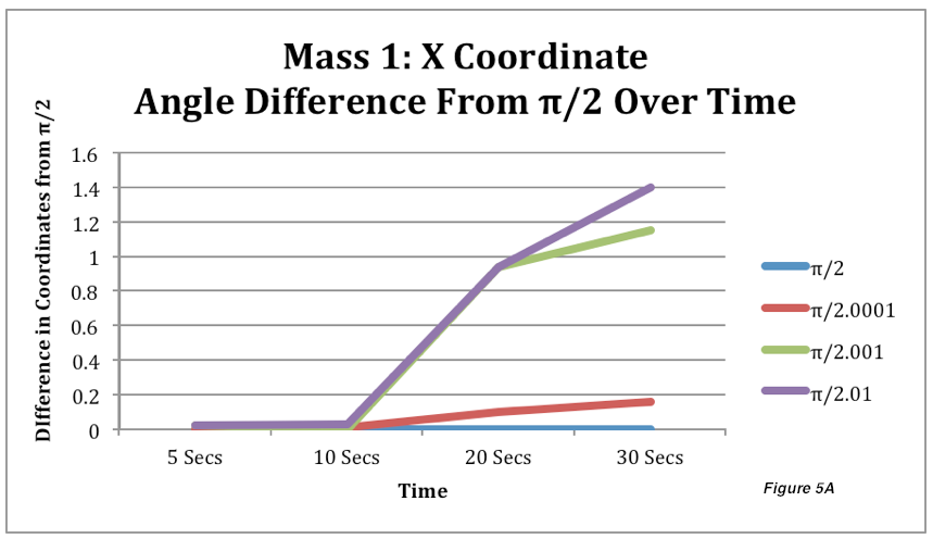
Graph showing the difference between the mass 1 X-coordinate of the control and that of the other initial starting angles.
|
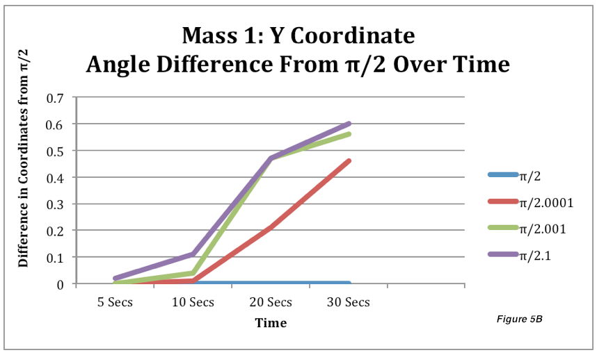
Graph showing the difference between the mass 1 Y-coordinate of the control and that of the other initial starting angles.
|
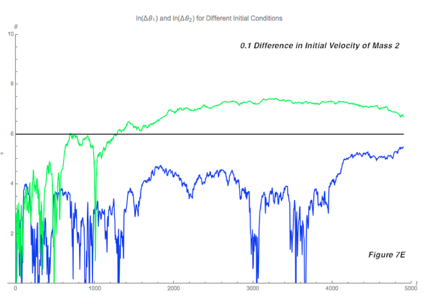
3) Finally, I plotted the difference between the angles of mass one and mass two of two double pendulums with different initial velocities (of the second mass) over time. I varied the velocities by 0.0001, 0.001, 0.01, and 0.1. These graphs also increased over time, albeit not as steadily as the others. While I was only looking for high sensitivity to initial starting conditions, this graph also showed through its constant steep drops and climbs that a double pendulum is also topologically mixing and dense in periodic orbits. The trajectories that were far apart suddenly became arbitrarily close for a while, before suddenly diverging drastically from each other. For example, in Figure 7E, the angle difference between the first masses (green) climbs relatively steadily, but that of the second masses (blue) peaks and plummets, especially between 3000 and 4000 seconds. If the double pendulum was simulated and observed, the paths of the second mass would appear to be the same when the differences reach 0 (appear – since it is most likely not that the paths are identical, but rather that the computer cannot differentiate between such small deviations) during the 3000-4000 seconds for a while, before suddenly dramatically diverging from each other. Apart from that, the differences still increased overall, showing the sensitivity of a double pendulum.
Conclusion
In conclusion, my entire hypothesis was proven correct. The double pendulum was highly sensitive to initial starting conditions, as shown by the increasing difference between its angles and coordinate positions between a control and variations in initial velocities and angles of 0.0001, 0.001, 0.01, and 0.1. The paths became more and more different over time, and if left to continue, would end up being significantly different from another double pendulum, even if the difference at the beginning was as small as a ten thousandth. Since I had already established through research that a double pendulum was topologically mixing and had a dense periodic orbit, and through my experiment it was shown to be also highly sensitive to initial starting conditions, my hypothesis was verified and a double pendulum was ultimately proven to be a chaotic system.
Overall, I think my experiment was quite successful. I kept my controlled variables consistent by using my computer for calculation, Mathematica for animation, Excel for tables and line graphs, and gave the terms not altered as an initial starting condition (such as rod length and mass weight) the same numeric value throughout the experiment. The independent variables of initial starting angles and velocities were changed to alter the dependent variable, the path of the double pendulum (from which I obtained the coordinate positions and angle differences). Compared to expected results from books and websites, my results yielded the same conclusion – a double pendulum is indeed a chaotic system. If I could redo the project, I would alter my experiment to include testing topological transitivity and dense periodic orbits, and also perform the same tests I did on a double pendulum to a single pendulum so I would have a better comparison. It would also be interesting to use a physical double pendulum and see how it actually looks in real life. Some possible sources of error could be inaccurate rounding of the decimal points in the coordinate plane table or typos when running the script. Nonetheless, I think the project went quite well and it was a very fun and educational experience!
Overall, I think my experiment was quite successful. I kept my controlled variables consistent by using my computer for calculation, Mathematica for animation, Excel for tables and line graphs, and gave the terms not altered as an initial starting condition (such as rod length and mass weight) the same numeric value throughout the experiment. The independent variables of initial starting angles and velocities were changed to alter the dependent variable, the path of the double pendulum (from which I obtained the coordinate positions and angle differences). Compared to expected results from books and websites, my results yielded the same conclusion – a double pendulum is indeed a chaotic system. If I could redo the project, I would alter my experiment to include testing topological transitivity and dense periodic orbits, and also perform the same tests I did on a double pendulum to a single pendulum so I would have a better comparison. It would also be interesting to use a physical double pendulum and see how it actually looks in real life. Some possible sources of error could be inaccurate rounding of the decimal points in the coordinate plane table or typos when running the script. Nonetheless, I think the project went quite well and it was a very fun and educational experience!
